Getting started
For illustration purpposes, let’s go step by step through a simple example where a slotted disk rotates through a (circle-shaped) mesh. The rotation of the slotted disk is governed by the solid body rotation
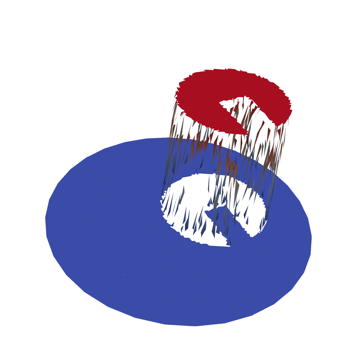
The slotted disk is represented on a set of particles, see the following picture of what could be the initial particle field.

Our objective is to project the scattered particle representation of the (rotating!) slotted disk onto a FEM mesh in such a way that the area is preserved (i.e. mass conservation). Apart from conservation, we certainly want the particle-mesh projection to be accurate as well. To achieve this, the PDE-constrained particle-mesh projection from Maljaars et al [2019] is used. This projection is derived from the Lagrangian functional
An in-depth interpretation and analysis of this functional and the optimality system that results after taking variations with respect to \(\left(\psi_h, \lambda_h, \bar{\psi}_h \right) \in \left(W_h, T_h, \bar{W}_{h} \right)\), can be found in the aformentioned reference.
First, let’s import the required tools from leopart:
from leopart import (
    particles,
    advect_rk3,
    PDEStaticCondensation,
    FormsPDEMap,
    RandomCircle,
    SlottedDisk,
    assign_particle_values,
    l2projection,
)
And import a number of tools from dolfin and other libraries:
from dolfin import (
Expression,
Point,
VectorFunctionSpace,
Mesh,
Constant,
FunctionSpace,
assemble,
dx,
refine,
Function,
assign,
DirichletBC,
)

from mpi4py import MPI as pyMPI
import numpy as np

comm = pyMPI.COMM_WORLD
Next is to further specify the geometry of the domain and the slotted disk. Furthermore, we import the disk-shaped mesh, which is refined twice in order to increase the spatial resolution
(x0, y0, r) = (0.0, 0.0, 0.5)
(xc, yc, r) = (-0.15, 0.0)
(r, rdisk) = (0.5, 0.2)
rwidth = 0.05
(lb, ub) = (0.0, 1.0)

# Mesh
mesh = Mesh("./../../meshes/circle_0.xml")
mesh = refine(refine(refine(mesh)))
The slotted cylinder is created with the SlottedDisk class, this is nothing more than just a
specialized dolfin.UserExpression and provided in the leopart package just for
convenience:
psi0_expr = SlottedDisk(
    radius=rc, center=[xc, yc], width=rwidth, depth=0.0, degree=3, lb=lb, ub=ub
)
The timestepping parameters are chosen such that we precisely make one rotation:
Tend = 2.0
dt = Constant(0.02)
num_steps = np.rint(Tend / float(dt))
In order to prepare the PDE-constrained projection, the function spaces \(W_h\), \(T_h\) and \(\bar{W}_h\) are defined. Note that \(\bar{W}_h\) is defined only on the mesh facets. Apart from the function space definitions, we also set a homogeneous Dirichlet boundary condition on \(\bar{W}_h\), and we define the advective velocity field.
W = FunctionSpace(mesh, "DG", 1)
T = FunctionSpace(mesh, "DG", 0)
Wbar = FunctionSpace(mesh, "DGT", 1)

bc = DirichletBC(Wbar, Constant(0.0), "on_boundary")

(psi_h, psi_h0, psi_h00) = (Function(W), Function(W), Function(W))
psibar_h = Function(Wbar)

V = VectorFunctionSpace(mesh, "DG", 3)
uh = Function(V)
uh.assign(Expression(("-Uh*x[1]", "Uh*x[0]"), Uh=np.pi, degree=3))
We are now all set to define the particles. So we start with creating a set of point locations
and setting a scalar property that, for instance, defines the concentration. Note that leopart
comes shipped with a number of particle generators, of which the RandomCircle method is just
one.
x = RandomCircle(Point(x0, y0), r0).generate([750, 750])
s = assign_particle_values(x, psi0_expr)
…and define both the particle object and a particle-advection scheme (in this case a Runge-Kutta 3 scheme)
The optimality system that results from minimizing the Lagrangian can be represented as a 3x3 block matrix at the element level
The ufl-forms for the different contributions in this algebraic problem can be obtained with the
FormsPDEMap class. Furthermore, we feed these forms into the PDEStaticCondensation
class that will be used for the acutal projection:
Note that in the snippet above, the \(\zeta\) parameter which penalizes over and undershoot is set to a value of 30. Other than scaling this parameter with the approximate number of particles per cell, there is (as yet) not much more intelligence behind it).
We are almost ready for running the advection problem, the only thing which we need is an initial
condition for \(\psi_h\) on the mesh. In order to obtain this mesh field from the particles,
the bounded \(\ell^2\) projection that is available in leopart is used, i.e.
lstsq_psi = l2projection(p, W, 1)

lstsq_psi.project(psi_h0, lb, ub)
assign(psi_h00, psi_h0)
This results in the initial mesh field as shown below:
Now we are ready to enter the time loop and solve the PDE-constrained projection in every time step for reconstructing a conservative mesh field \(\psi_h\) from the moving particle field.
step = 0
t = 0.0
area_0 = assemble(psi_h0 * dx)

while step < num_steps:
    step += 1
    t += float(dt)

    if comm.Get_rank() == 0:
        print(f"Step {step}")

    ap.do_step(float(dt))

    pde_projection.assemble(True, True)
    pde_projection.solve_problem(psibar_h, psi_h, "mumps", "default")

    assign(psi_h0, psi_h)
Finally, we want to check if we indeed can keep our promise of being conservative and accurate, so let’s check by printing:
area_end = assemble(psi_h * dx)
num_part = p.number_of_particles()
l2_error = np.sqrt(abs(assemble((psi_h00 - psi_h) * (psi_h00 - psi_h) * dx)))
if comm.Get_rank() == 0:
    print(f"Num particles {num_part}")
    print(f"Area error {abs(area_end - area_0)}")
    print(f"L2-Error {l2_error}")
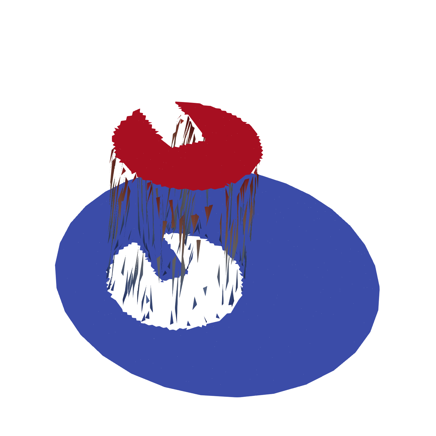
That’s all there is! The code for running this example can be found on Bitbucket. Just to convince you that it works, this is the reconstructed mesh field at \(t=1\), after a half rotation: